Building the Digital Abacus, an Open-Source Mathematical Modeling App
Part 1: The Automatic Constraint Solver
Editor’s note: the scope of this blog is expanding. Going forward, some posts will discuss human-programming tools, and others will cover my adventures as a programmer who is a human (so you see, the name ‘Human Programming’ is backwards compatible). This series is the first in the latter category. I write with the same audience in mind — people interested in human-computer interaction, web tools, programming interfaces, and personal development. With that said, I’m confident you’ll enjoy this series exploring the inner workings of an experimental math tool: the Digital Abacus.
Introduction
In February of 2023, I was holed up in San Bruno, CA, deep in development of a flowchart-powered developer tool called InstructionKit.
My cofounder Chris and I were looking to bootstrap, so we needed side gigs. Chris was already working part-time with Hack Club to produce his amazing game SineRider (check it out), and would soon connect me with Paul Dancstep, who was looking for help with his project called the Digital Abacus.
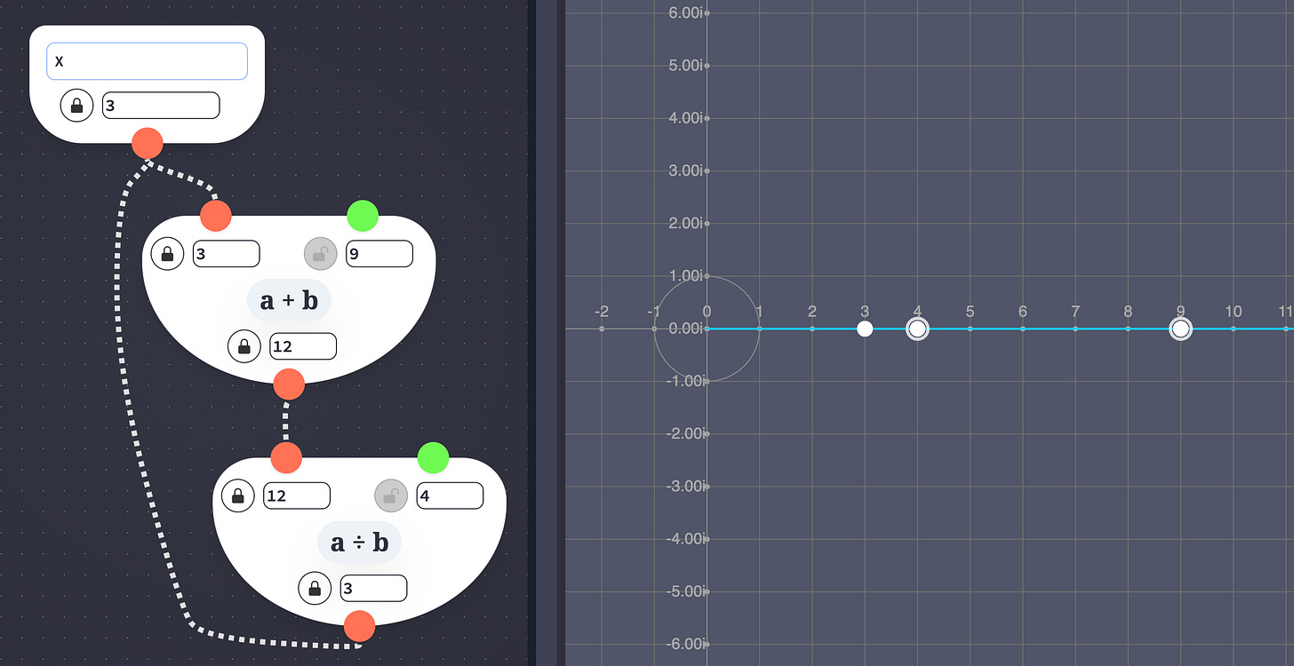
As Paul explained, he and a team of mathematicians were building a tool for solving math problems, to be used by students and professionals alike. Something that would look like this:
There would be two interfaces: on the left, a flowchart with nodes and edges representing operators and constraints, and on the right, a plot showing the live-updating real and imaginary coordinates of every input-, intermediate-, and output-value in the system. The user could directly drag and manipulate values from either view, so they could construct reusable interactive tools to help them model real-world systems (see this lecture for some conceptual background).
This project sounded like a perfect match for me given my experience building InstructionKit, so I joined and spent a fantastic three months working with the team to produce the version shown above (here is a demo and here is the source code).
I enjoyed this project so much that figured I should write about the tool’s unique technical design and the decisions that went into it. Eventually I decided to split things into a multi-part series, with the following sections:
Table of Contents
The Automatic Constraint Solver ← you are here
…
…And you’re coming up on part one. Enjoy!
Pt. 1: The Automatic Constraint Solver
Note: we refer to an arrangement of nodes and wires as a ‘construction’.
First I’ll describe the experience of building and interacting with a construction using the Digital Abacus Tool, then I’ll talk about the underlying state representation of a construction, and finally how the tool solves for dependent values.
An example construction: Euler’s Identity
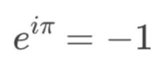
Say we want to model and explore Euler’s identity using our tool:
To do so, we drag the constants, e, pi, and i into the flowchart workspace. We connect pi and i to the input terminals of a Multiplier to yield the product i * pi. Finally we connect e and i * pi to the input terminals of an Exponentiator to yield the result, -1. Like so:
What makes this UI special?
Merely solving e^(i*pi) is not all that interesting; Google does a good enough job at that. What makes our tool here special is that we can see our values interacting in the complex plane. And, more importantly, we can drag our input values around, watching dependent values update instantly and continuously. By playing with the system, the user can understand the mechanics underlying the equation. Instead of being a single-shot calculation, our equation has become an explorable explanation.
We can even reverse dependencies in the construction to make the output a free variable and solve for one of the inputs, all with a couple of clicks (more on this soon).
The shape of the constraint graph
So how does this work under the hood? First, we need to store all of the values and constraints within the construction.
We do so in a graph data structure (called the RelGraph in the code). The RelGraph (short for relation-graph) is the single source of truth for all information about a particular model, including the shape of a model (what components it has in the flowchart) as well as the state of values within a model.
Vertices and Edges
The RelGraph contains Vertices and Edges. A Vertex (code) represents a numerical value with real and imaginary parts. With respect to the system as a whole, a Vertex could be an input, output, or intermediate value.
An Edge (code) represents a constraint between two or more values. For example, connecting two values by a wire in the flowchart UI corresponds to an equality constraint Edge in the RelGraph. Continuing our example, let’s see how Vertices and Edges work together:
A concrete example: the RelGraph for Euler’s Identity
The image below shows the RelGraph created for our construction of Euler’s Identity. Vertices/values are blue (and are given arbitrary uppercase letters as IDs for the sake of this diagram), while Edges/constraints are green. As you can see, a RelGraph is a hypergraph where Edges can connect multiple Vertices. The messy image further below illustrates how this RelGraph corresponds to the nodes and wires in the flowchart UI.
Note that our construction has some extra Vertices at the incoming and outgoing terminals of our Multiplier and Exponentiator. That’s because these operators come with their own input and output Vertices. Wiring up two values does not merge them, rather it creates an additional equality constraint between them.
Operators are reversible, so users can solve for different variables
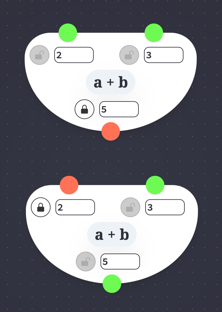
An important affordance of the system is that every single operator can run in reverse; you can turn what used to be an output into an input. For example, you can unlock the sum value below an Adder, give up control of one of the addends, and suddenly you can run the Adder in reverse, effectively as a Subtractor.

Reversing multiple operators at a time
The UI makes it easy to reverse multiple operators at once; the user can lock and unlock disparate Vertices, and the tool will find a path of Edges (operators and equality-constraints) between them, reversing all of those edges simultaneously.
This allows the user to quickly solve for different variables in a system. For example, a mechanical engineer who is modeling pressure with a headset strap might wonder “if I set pressure and head size to these constants, what is the resulting optimal strap length?” Later, once a strap length is selected, they might free up the head-size variable, allowing them to ask “given this strap length, what is the smallest head size that yields at least some minimum amount of pressure?”
How the RelGraph reaches equilibrium
The screenshots and renderings above show a RelGraph in equilibrium, but the RelGraph is not always in equilibrium. When you first connect an operator to some values, or when you drag a value around, the system will be in a temporary disequilibrium, then will iteratively march towards a solution.
This march happens because the RelGraph is scheduled to regularly update its values (code). These updates are delegated to the RelGraph’s Edges; each edge updates its dependent Vertex’s value in an attempt to bring the Edge’s constraint closer to being satisfied. For example, an equality constraint spanning from a 4 to a 3 might update the 3 value to a 3.02 in a single update cycle, then on to 3.04 and 3.06 and so on, such that equality between the two values is closer to being satisfied.
Depending on the speed and granularity of updates that you’ve set, you can see this march in real time as the system solves itself.
Note: the way in which the system marches towards equilibrium is abstracted away from the structure of the graph itself. The team wrote a few versions of those update functions (differential, ideal, and iterative) which live in this folder. We’re currently using the iterative updaters within the file iterative.ts, which is why the RelGraph doesn’t instantaneously reach equilibrium.
Reaching equilibrium can fail
Since you can create cyclic constructions where a value indirectly relies on itself, not every construction is guaranteed to reach equilibrium. Some systems will result in values that spin around in circles, or that gradually spiral towards equilibrium, or that run off towards infinity.
Note: The team added some special behavior to the updaters in iterative.ts to help guide cyclic constructions towards stable equilibria, which involves calculating the differential of a dependent value with respect to the input being manipulated. A full explanation is out of the scope of this post.

Representing composite operations
So far we’ve covered the basics of the constraint solver; now on to my favorite part: composite operations.
The Digital Abacus Tool started with only four primitive operators: Adder, Multiplier, Exponentiator, and Conjugator. These building blocks can be used to make basically any mathematical function [citation needed], but we also wanted to give the user a wider menu of operators to work with. Rather than implement update-functions for every single operator we wanted, we decided to support Composite Operations, meaning that a single node in the flowchart could encapsulate multiple primitive operations in the RelGraph. This would let us add things like logarithms and trig functions.

We discussed two ways to enable composites: One option was to add multiple Edges and Vertices to the main RelGraph graph per composite operation. Another option was for each composite operation to contain its own subgraph. Each subgraph would itself be a RelGraph, and could contain any of the primitive operators listed above, or could recursively contain more subgraphs (spoiler, we chose this approach).
The subgraph pattern for composite operations
Here’s how subgraph-based composite operations work: suppose we have a Subtractor within our main RelGraph, with input values 5 and 3. When it’s time for the Subtractor to update, that Subtractor pulls the 5 and the 3 down from the main RelGraph into its subgraph, then runs its subgraph’s update function (which contains a reversed Adder), and finally pushes the result, 2, back up into the main graph. Here’s the code that runs those nested updates.
We chose the subgraph approach for a few reasons. First of all, it gave us a nice pattern to use for creating composites: We could create a composite in the UI, then serialize it and store it as a configuration file associated with that particular composite’s sidebar menu item (example configuration). This serialized configuration represents the initial equilibrium state of the composite operation’s subgraph, and can be deserialized to create a fresh copy of the composite operation whenever a user drags a new composite node into the flowchart.
The subgraph pattern also simplifies batch operations. Deleting a composite is easy: since you just delete its subgraph, you don’t have to go searching the main RelGraph for related Vertices and Edges.
Coming soon: custom composite operations
Some small updates to the UI could allow users to build and edit their own composite operations using the exact same flowchart and plot UIs, giving users a personal component library of math functions relevant to their work. This would be relatively simple, since the RelGraph powering the entire UI could easily be swapped out for the scoped RelGraph that defines any given composite.
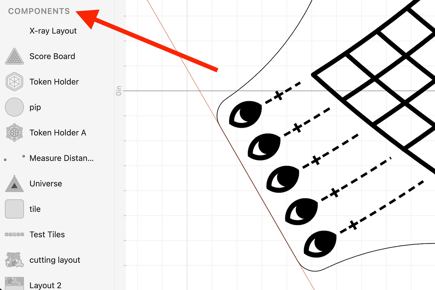
This could look similar to Cuttle’s component system, shown below, where user-defined components are listed in the left sidebar and can be dragged into the current work area.

Up Next
Thank you for reading. If you haven’t already, please subscribe below for future updates, including the upcoming post: Building the Digital Abacus pt. 2: Reactivity & Persistence.
P.S. I worked on this project in my capacity as a product development contractor and am open to new clients. Also the Digital Abacus is looking for funding to continue pushing the boundaries of free & open-source math tools. Feel free to reach out for either.
Best,
Daniel Sosebee


